Sequential Minimal Optimization
The iterative algorithm Sequential Minimal Optimization (SMO) is used for solving quadratic programming (QP) problems. One example where QP problems are relevant is during the training process of support vector machines (SVM). The SMO algorithm is used to solve in this example a constraint optimization problem. John Platt proposed this algorithm in 1998 and it was succesfully used since then. We describe here the basics of the algorithm in the light of big data.
Benefits and Drawbacks of QP Problems
The SVM training process is slow especially for big data. One of the reasons of being slow is that it requires a solution of an extremely large QP optimization problem. When considering N data points and N is a very large number we have a true big data problem. This is because the QP running time is O(N3) in the worst case. Although this problem can not directly be solved SMO is one approach of dealing with large quantities of datasets. It requires an amount of memory that is linear in the training set size N. That enables SMO to handle such large datasets using techniques described below.
SMO Goal and SVM Formulation
The SMO algorithm is a successful attempt to improve the training process of SVMs that was previously based on so-called “chunking”. The goal of the SMO algorithm is to return the alphas that satisfy the constraint optimization problem below. The constraints are given using a known description such as ‘subject to (s.t.)’. In terms of machine learning this is the actual inherent learning process. These alphas are called Lagrange multipliers. They play a key role to identify support vectors in our data.
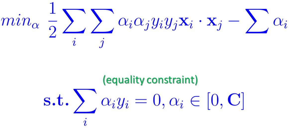
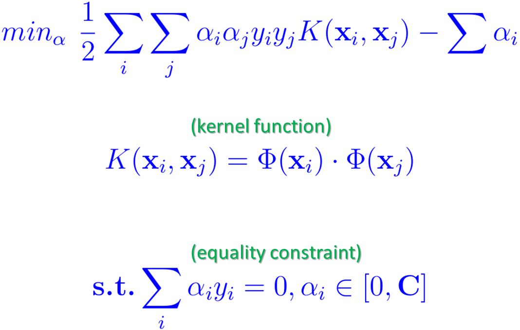
When working with non-linear SVMs a user chooses a Kernel function K in order to transform data into a higher dimension. Therefore we can exchange the dot product of x with the Kernel function K. The updated optimization problem is then as follows. It is sometimes also named as the ‘objective function’ or a ‘quadratic cost function’. But the inherent big data issue remains meaning that the quadratic form below involves a matrix that has a number of data elements to the square of the number of N training samples.
Instead of providing all alphas at once SMO is formulated as an iterative algorithm. It breaks this big QP optimization problem into a series of small QP optimization sub-problems (see Step One). Each sub-Problem is then solved analytically (see Step Two) until convergence (see Step Three). This analytical approach in the core of SMO avoids time-consuming numerical QP optimization techniques. Since large matrix computation is avoided, it scales between linear and quadratic in the training set size N depending on the data analysis problem. The SMO computation time is dominated by the evaluation of the SVM and thus it is faster for linear SVM problems and sparse datasets. In other words SMO spends most of the time evaluating the decision function instead of solving QP. That means it exploits very well large sparse datasets that contain a high number of zero elements.
SMO Step Zero
Before the algorithm starts the alphas need to be initialized with values. Then the next three steps are iterated until convergence.
SMO Step One
This step picks exactly two alphas from all n available alphas. This pair is one sub-problem mentioned above and represents the smallest possible optimization problem for the given problem. That means two Lagrange multipliers are involved because those Lagrange multipliers must obey the linear equality constraint shown above. The most promising pairs of alphas are picked by using certain heuristics. That means from the full vector of alphas just two are picked at a certain iteration. It is useful in order to accelerate the rate of convergence. In other words from the field of parallel computing this gives enormous speed-ups. Especially for big data sets it is very useful since there are n(n-1) possible choices for the pairs.
The first Lagrange multiplier is provided by the so-called “outer loop” of the SMO algorithm. This “outer loop” iterates over the whole training set. It checks each sample for violations of the so-called Karush-Kuhn-Tucker (KKT) conditions. These conditions are easy to compute per sample. If one sample violates the KKT conditions it is marked for requiring optimization.
SMO Step Two
This step only optimizes two alphas at a time in order to find optimal values for these two multipliers. Hence, these two alphas are (re-)optimized while all other remaining alphas stay constant. There need to be at least two alphas as the smallest set to optimize because there is an equality constraint given above. Hence, the minimal in SMO means exactly these two alphas. With two alphas this can be easily computed. It represents a closed-form solution that is fast to compute analytically. That means we need no “inner iteration” in this particular step using numerical QP optimization.
As a consequence the SMO is a very efficient algorithm since the sum in the formula above is literally just considering two ‘variables’ (i.e. alphas) at a time. Still the whole algorithm needs to solve more optimization sub-problems then. But each sub-problem in this step is so fast that the overall QP optimization problem can be quickly solved. With respect to big data also memory consumption is worth to consider. This step does not require another matrix storage for the full QP problem. Instead this step needs minor amount of memory to store 2 x 2 matrices at each iteration.
SMO Step Three
Repeat Step One and Step Two until the algorithm converges. The convergence criteria for the SMO algorithm are defined as Karush-Kuhn-Tucker (KKT) conditions. It means that SMO converges when all the Lagrange Multipliers (i.e. all alphas) satisfy this criteria. In other words the optimization problem is solved then. In practice one could define a user-defined tolerance to which degree really all alphas have to satisfy the KKT conditions.
It has been shown that the SMO algorithm is guaranteed to converge using the above criteria. A theorem outlined in detail here enables that a large QP problem can be actually broken down into a sequential order of smaller QP sub-Problems. This sequence that always add at least one violator of KKT conditions is then guaranteed to converge at some time.
SMO Implementation
One of the most famous libraries that implement the SMO algorithm is the LibSVM library. It represents also the de-facto standard library for SVMs.
More Information about Sequential Minimal Optimization
We recommend to watch the following video:
There is also the original technical paper named ‘Sequential Minimal Optimization: A Fast Algorithm for Training Support Vector Machines’ that is available here.
Follow us on Facebook: